
Unlocking Pairing-Based Cryptography with Elliptic Curves
Pairing-Based Cryptography Demystified: A Deep Dive into Elliptic Curves
Elliptic curves are central to modern cryptography, offering efficient, secure systems with smaller key sizes compared to traditional methods like RSA. But before diving into what they do, it’s helpful to understand what they are.
Elliptic curves are mathematical objects that allow us to define a special way of combining points — like a kind of addition. This simple operation hides a hard mathematical problem at its core, known as the elliptic curve discrete logarithm problem (ECDLP), which is what makes elliptic curves secure and useful in cryptography. Over time, we’ve learned to enhance their efficiency: we can change how points are represented (to speed up computations), or choose special types of curves that are optimized for advanced tools like pairings — powerful constructions used in advanced cryptographic protocols that allow you to verify that a computation was done correctly even when repeating the entire computation yourself would be impractical or impossible.
To understand why and how elliptic curves enable these tools, let’s start by defining them and discussing their geometric and algebraic properties, then explore how they underpin pairing-based cryptography and the construction of advanced cryptographic schemes.
Introduction to Groups, Subgroups and Finite Fields
This part is a little introduction to the concepts of Groups and Finite Field, essential for understanding Elliptic Curves.
Groups
A group $\mathbb{G}$ is a set of values containing a neutral element (often noted $0$) where an operation (often noted $+$) can be performed, with the following property:
$$\forall x \in \mathbb{G}, \exists y \in \mathbb{G} \text{ s.t. } x + y =0.$$
The meaning of this is that every element in the group has its opposite. By construction, every result of the group operation lies also in the group; we call this property being closed.
Examples
What is a group
-
$\mathbb{R}$ is a group for the operation "addition"
-
$\mathbb{R}/{0}$ ($\mathbb{R}$ without $0$) is a group for the operation "multiplication" —we remove $0$, because it has no inverse in $\mathbb{R}$
-
$\mathbb{Z}$ (the set of every integer—positive or negative—) is a group for the operation "addition"
-
👕 T-shirt orientations with the operation “apply one transformation after another”:
-
The four elements are: do nothing ($D$), inside out ($I$), backwards ($B$), inside out and backwards ($IB$)
-
Identity: wearing it normally ($D$)
-
Every orientation(=element of the group) has an inverse: e.g., $I$ + $I$ = $D$, $B$+ $B$ = $D$, etc.
-
Combining two transformations gives another valid orientation: e.g., $B$ + $I$ = $IB$ — the group is closed
Your clumsy morning dressing habits form a group!
-
What is not a group
- $\mathbb{Z}/{0}$ ($\mathbb{Z}$ without $0$) is not a group for the operation "multiplication" —only $1$ and $-1$ have an inverse in $\mathbb{Z}/{0}$, every other inverse will not lie in $\mathbb{Z}/{0}$ because they are not entire values
- $\mathbb{N}$ (the set of every positive integer) is not a group for the operation "addition" —only $0$ has an opposite in $\mathbb{N}$, every other opposite will not lie in $\mathbb{N}$ because they are not positive values
Subgroup
Inside a group, another group can be hidden!
A subgroup is a smaller set of elements from a group that still behaves like a group itself. It must include the identity, be closed under the operation, and contain inverses for all its elements.
For example:
- $2\mathbb{Z}$ (the set of even values in $\mathbb{Z}$) is a subgroup of $\mathbb{Z}$ for the addition, because:
- the opposite of any even value is an even value (and so in $2\mathbb{Z}$)
- the addition of two even values gives an even value
- $0$ is an even value
👕 Or take the t-shirt transformation group:
-
The full group includes these operations:
Do nothing, ($D$), inside out ($I$), backwards ($B$), `inside out and backwards ($IB$). -
The subgroup [Do nothing, ($D$), inside out ($I$)] also forms a group on its own:
-
Doing nothing is the identity,
-
Flipping inside out twice brings you back,
-
It’s closed under the operation of combining these actions.
Yes, your wardrobe knows abstract algebra.
-
(Finite) Fields
A field is like a supercharged group: it has not just one, but two operations — usually addition ($+$) and multiplication ($×$).
It must satisfy the following:
- The set forms a group under addition (with identity $0$)
- The set without $0$ forms a group under multiplication (with identity $1$)
- Multiplication is distributive over addition: $a \times (b + c) = a \times b + a \times c$
The most familiar field is $\mathbb{R}$ (real numbers), where:
- You can add, subtract, multiply, and divide (except by $0$)
- The result always stays in $\mathbb{R}$
But fields don’t have to be infinite!
There are finite fields too — and they’re absolutely everywhere in cryptography 🔐
A very simple example is the field $\mathbb{F}_5 = [0, 1, 2, 3, 4]$, where:
- All operations are done modulo $5$
- You can still add, subtract, multiply, and (except for $0$) divide!
2 + 4 = 1 mod 5     ✅
3 × 4 = 2 mod 5     ✅
2⁻¹ = 3 mod 5       ✅ because 2 × 3 = 6 = 1 mod 5
We can extend this principle to any prime number (we need the modulus to be prime for reasons we won't go into here), and we note $\mathbb{F}_p$ the finite field consisting of the integers modulo $p$, and where the addition and the multiplication are done modulo $p$.
Definition of an Elliptic Curve
An elliptic curve $E$ over a field $\mathbb{F}_p$ is noted $E(\mathbb{F}_p)$ and is defined by the set of the points of coordinates $(x,y) \in \mathbb{F}_p^2$ respecting a Weierstrass equation of the form:
$$ y^2 = x^3 + ax + b $$
where:
- $a, b \in \mathbb{F}_p$.
An elliptic curve has the following form:
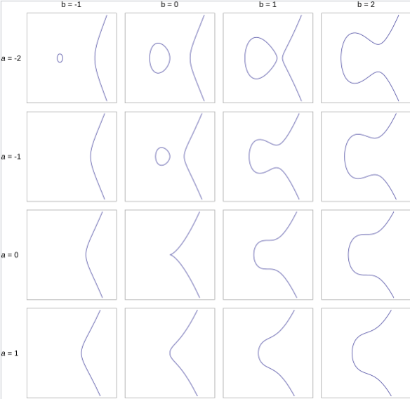
Here we just take $a, b \in [ -2, 1 ]$ to illustrate, but they can take any value in $\mathbb{F}_p$. We have to note that the previous graphical representations are valid only if we consider the coordinates in $\mathbb{Q}$, indeed, due to the modulo property of the finite fields, the graphical representation with finite fields is much less clear and ordered.
The curve must be non-singular, which means it has no cusps or self-intersections. This is ensured by the discriminant:
$$ \Delta = -16(4a^3 + 27b^2) $$
To have a valid elliptic curve:
$$ \Delta \neq 0 $$
This condition guarantees that the curve is smooth—no singular points—so the tangent at any point is well-defined. For example in the case $(a,b) = (0,0)$, the curve is not smooth because we have a peak, and we cannot draw the tangent of this peak, so we cannot compute the double of this point (see the next section for explanations of the "double" operation)), which makes this curve not an elliptic curve.
Working over Finite Fields
In cryptography, we typically work over finite fields $\mathbb{F}_p$, where $p$ is a prime.
This finite setting ensures that the number of possible $x$ and $y$ values is finite, crucial for practical cryptographic applications. We call this finite field the base field of the curve.
Geometric Group Law: Elliptic Curve Operations
A remarkable property of elliptic curves is that the set of points on the curve forms an commutative group under a special addition operation. Let’s understand this geometrically.
Addition of Points
- Adding two distinct points $P$ and $Q$:
- Draw a straight line through $P$ and $Q$. This line will intersect the elliptic curve at a third point, $-R$.
- Reflect $-R$ across the $x$-axis to get the sum $P + Q = R$.
-
Doubling a point $P$:
- When $P = Q$, consider the tangent to the curve at $P$.
- The tangent intersects the curve at a third point $-R$.
- Reflect $-R$ across the $x$-axis to obtain $2P=R$.
The Identity Point (Point at Infinity)
The elliptic curve group has a neutral element, often denoted $\mathcal{O}$ or the “point at infinity.” Geometrically, this is the “intersection” of the vertical line in the projective plane, ensuring a complete group structure:
- For any point $P$, $P + \mathcal{O} = P$.
- In practice, $\mathcal{O}$ is treated as a special symbol outside the usual $(x,y)$ coordinate system.
You can see it as a magical point "outside" of the graph, but on the curve at the very top or at the very bottom. Indeed, when we add two points with the same $x$-coordinates but with different $y$-coordinates, they are vertically perfectly aligned, and then the line passing by these points doesn't cut the elliptic curve, except of course at this point at infinity. We can then say that $P + (- P) = \mathcal{O}$.
The Generator Points
Any elliptic curve defined on a finite field $\mathbb{F}_p$ has a finite number of elements (=points). We call this number of elements the order of the curve, and we denote it by $|E|$.
We can always extract from $E$ a subgroup $\mathbb{G}$ of order $r$, with $r$ prime, that allows us to preserve the properties of the elliptic curve. We call $\mathbb{F}_{r}$ the scalar field of this subgroup —to not confuse with the base field of the curve—. We can now denote $k$ repeated additions of a point $P \in \mathbb{G}$ by $k \times P$, with $k \in \mathbb{F}_r$.
Every prime order subgroup is cyclic, which means that it can be generated by one element —noted commonly $G$—, which means that adding successively $G$ to itself gives every point of $\mathbb{G}$, until reaches again $G$. This generator is not unique; this is why we talk about a generator.
If $G$ is a generator of $\mathbb{G}$, then
$$ \mathbb{G} = [G, 2 G, 3 G, 4 G, \cdots, (r-1) G, r G = \mathcal{O}] $$
Point Representation: Affine and Projective Coordinates
Affine Coordinates
In the basic Weierstrass form, points on the curve are usually written as pairs $(x, y)$ such that $y^2 = x^3 + ax + b$.
It is a classical and intuitive representation, storing an elliptic curve point using just two field elements. But let’s see what happens computationally when we add such points.
The exact formula to compute $P + Q = R$ is the following —don't panic, you don't really have to read it, we'll come back to it right after:
Case 1: $P \neq Q$
Let
$$ \lambda = \frac{y_2 - y_1}{x_2 - x_1} $$
The new coordinates:
$$ R_x = \lambda^2 - x_1 - x_2 $$
$$ R_y = \lambda (x_1 - R_x) - y_1 $$
Case 2: $P = Q$ (Point Doubling)
If $y_1 \neq 0$, let
$$ \lambda = \frac{3x_1^2 + a}{2y_1} $$
The new coordinates:
$$ R_x = \lambda^2 - 2x_1 $$
$$ R_y = \lambda (x_1 - R_x) - y_1 $$
Point at Infinity
If $P = -Q$ (i.e., $x_1 = x_2$ and $y_1 = -y_2$), then:
$$ P + (-P) = \mathcal{O} $$
We can see that there are some divisions in these formulae (in $\lambda$ especially). Divisions are costly in finite fields—they take much more time than multiplications or additions, and we generally seek to minimize their usage. This is why we introduced:
Projective Coordinates
Instead of performing costly divisions for every addition, we defer them by introducing a third coordinate, representing the denominator. This allows us to batch divisions until the final result is needed. This lets us delay the division until the very end — either when we no longer need the point, or when we need its explicit (affine) coordinates. We trade many small divisions for a single, possibly more complex one at the end — which is generally much faster overall.
We will not show you the new formulae for the addition of projective points —the calculations are frightening— but instead an intuition of how it works.
Let us consider computing $\frac{a}{b} + \frac{c}{d}$, and that the divisions are costly. Doing the computation in the classical way (first dividing and after adding) costs two divisions and one addition. Instead, we can reduce the cost to three multiplications, one addition, and one division with the following method:
$$ \frac{a}{b} + \frac{c}{d} = \frac{a \times d}{b \times d} + \frac{c \times b}{b \times d} = \frac{a \times d + c \times b}{b \times d} $$
Here, we "waste time" calculating some multiplications that were not there originally, but we save the cost of a division. As a reference, the cost of a division compared to the cost of a multiplication can vary from a factor of $5$ to more than $100$ —this is an order of magnitude, and must not be taken as a real proven value. It depends on the implementation, the finite field, the computing power of the machine, and many others.
We can also notice that this optimization is even better the more additions we have. If we have two fraction additions instead of one, then the cost goes from three divisions and two additions to eight multiplications, two additions, and one division:
$$ \frac{a}{b} + \frac{c}{d} + \frac{e}{f} = \frac{a \times d + c \times b}{b \times d} + \frac{e}{f} \ = \frac{(a \times d + c \times b) \times f}{b \times d \times f} + \frac{e \times b \times d}{b \times d \times f} \ = \frac{a \times d \times f + c \times b \times f + e \times b \times d}{b \times d \times f} $$
Let's suppose now that we are doing some fraction additions, but we do not know when we stop it, and when we will need the real result value of these computations. Then we do not divide by the denominator each time; instead, we carry the divisor along, storing and accumulating it to make the division operation at the very end, exactly as in our very previous example with 2 additions instead of 1.
Concretely, projective points are represented by three coordinates: $(X, Y, Z)$, where:
$$ x = \frac{X}{Z}, \quad y = \frac{Y}{Z} \text{ when } Z\neq 0 $$
$\mathcal{O}$ has its $Z$ coordinate equal to $0$.
Without going into details, the third coordinate is used to store the terms of the division, as in the previous examples with the denominator. It is at the end, when we decide to move from projective form to affine form, that the division takes place.
We can push the optimization even further using a specialized form of projective coordinates known as the Jacobian representation, where the coordinates are defined as:
$$ x = \frac{X}{Z^2}, \quad y = \frac{Y}{Z^3} \text{ when } Z\neq 0 $$
The calculations are even more complex, but also faster and more efficient.
Choosing Representations
-
Affine:
Best for understanding and small-scale experimentation. Intuitive and minimal, but costly in practice due to field inversions during point addition or doubling. -
Projective:
Improves performance by removing the need for costly divisions during intermediate operations. Ideal when many additions are involved, as in scalar multiplication. -
Jacobian:
A special form of projective coordinates that optimizes point doubling, the most frequent operation in scalar multiplication. Common in cryptographic implementations for its speed/memory tradeoff.
Comparison: Affine vs Projective vs Jacobian Coordinates
| Representation | Coordinates | Pros | Cons |
|---|---|---|---|
| Affine | $(x, y)$ | Simple, intuitive | Requires division for every add/double |
| Projective | $\left(\frac{X}{Z}, \frac{Y}{Z}, Z\right)$ | No divisions during operations | More complex formulas, extra coordinate |
| Jacobian | $\left(\frac{X}{Z^2}, \frac{Y}{Z^3}, Z\right)$ | Faster doubling; no divisions during operations | More memory; requires conversion for output |
The Elliptic Curve Discrete Logarithm Problem (ECDLP)
The security of elliptic curve cryptography relies on the Elliptic Curve Discrete Logarithm Problem (ECDLP):
Given:
- $G$ (a known generator point),
- $P = kG$ (a point obtained by adding $G$ to itself $k$ times).
Problem: Find $k$.
The naive approach—repeatedly adding $G$ until reaching $P$—works here only because $k=5$ is tiny. For a 256-bit $k$, this would take longer than the age of the universe! This algorithm has a time complexity of $O(|E|)$, which is the worst possible case.
Even with the most advanced known algorithms, solving the ECDLP on carefully chosen curves over large fields remains infeasible. This makes elliptic curve cryptography both secure and efficient.
The best known generic algorithm is Pollard’s Rho, a probabilistic method with a complexity of $O\left(\sqrt{|E|}\right)$. For a curve with $2^{256}$ points, solving the ECDLP would require approximately $2^{128}$ operations—well beyond current computational capabilities.
This hard-to-solve problem forms the foundation of many cryptographic protocols, much like the discrete logarithm problem in finite fields. If someone knows the secret scalar $k$, they can compute things efficiently (like generating a public key or decrypting a message). But someone who doesn’t know $k$ faces a prohibitive computational cost.
Introduction to Pairing-Based Cryptography
The inner construction of pairings is complex, highly technical, and beyond the scope of this blog post.
What is a Pairing?
A pairing is a special kind of function—called a bilinear map:
$$ e: G_1 \times G_2 \rightarrow G_T $$
where:
- $G_1$ and $G_2$ are (sub)groups of points on elliptic curves.
- $G_T$ is a multiplicative group (not elliptic-curve-based) in a finite field extension.
The key property is bilinearity:
For all scalars $a, b$ and all points $P \in G_1$, $Q \in G_2$:
$$ e(aP, bQ) = e(P, Q)^{ab} $$
This leads to several useful properties:
-
$\forall P, P' \in G_1,\ Q \in G_2$:
$$ e(P + P', Q) = e(P, Q) \times e(P', Q) $$
-
$\forall P \in G_1,\ Q, Q' \in G_2$:
$$ e(P, Q + Q') = e(P, Q) \times e(P, Q') $$
-
$\forall P \in G_1,\ Q \in G_2,\ \alpha \in \mathbb{Z}$: $$ e(\alpha P ,Q) = e(P, \alpha Q) = e(P, Q)^\alpha $$
Why are Pairings Important?
Pairings are not used to break ECDLP, but to verify relationships involving secrets, especially when those secrets remain hidden—like confirming a signature without seeing the private key.
For example, suppose you have:
- A generator $G \in G_1$,
- A generator $G' \in G_2$,
- A public point $Q = \alpha \times G'$ in $G_2$ (with unknown $\alpha$),
- A point $P$ in $G_1$ claimed to be $\alpha \times G$.
You can verify this claim without knowing $\alpha$ by checking:
$$ e(P, G')\ \stackrel{?}{=}\ e(G, Q) $$
Why does this work?
Because $G_1$ is cyclic, we can consider $P$ as the generator $G$ added to itself a certain number of time (claimed to be $\alpha$), let's say $\beta$ times: $P = \beta \times G$. Checking $$e(P, G')\ \stackrel{?}{=}\ e(G, Q)$$ is the same as checking $$e(\beta \times G, G')\ \stackrel{?}{=}\ e(G, \alpha G')$$ which leads to check $$e(G, G')^\beta\ \stackrel{?}{=}\ e(G, G')^\alpha$$ and so $$\beta\ \stackrel{?}{=}\ \alpha.$$
This trick is used all over modern cryptography.
Pairings enable advanced constructions such as:
- 🔑 Identity-Based Encryption (IBE) — where public keys are derived from identities like email addresses.
- ✍️ Short Signatures, like BLS (used in Ethereum 2).
- 🔐 Attribute-Based Encryption, enabling fine-grained access control.
These work because pairings allow the system to test relationships between secrets without revealing them.
Pairing-Friendly Curves: BLS12-381 and BLS12-377
BLS12-381 and BLS12-377 are part of a family of pairing-friendly elliptic curves, specifically designed for modern cryptographic protocols that rely on efficient pairings — such as zero-knowledge proofs and BLS signatures.
Both curves belong to the Barreto–Lynn–Scott (BLS) family, which defines curves with a particular structure, chosen to make pairings efficient while keeping security high.
Let’s break this down slowly.
A First Property: The Curve Equation
In the BLS family, all curves are defined with a simplified elliptic curve equation where the $a$ coefficient is set to zero. That gives us:
$$ y^2 = x^3 + b $$
This simplification (setting $a = 0$) is not arbitrary — it allows certain optimizations in implementation, especially when working in fields of large prime characteristic.
The Magic Parameter: $\mathrm{x}$
Now, how are these curves actually built?
Without going too deep into the math, the core idea is that the whole curve — and everything around it — is built from one main parameter, usually denoted $\mathrm{x}$ (important: this is not the same as the $x$ in the curve equation above).
From this parameter $\mathrm{x}$, we derive:
- the base field $\mathbb{F}_p$, which defines the "space" where the coordinates of our points live,
- the prime $r$ which defines the number of elements of the (subgroups of the) curve and then the scalar field
That’s the key: the curve itself doesn’t have a prime number of points, but we can isolate a subgroup of prime size. The parameter $\mathrm{x}$ is chosen in such a way that this subgroup has the right properties for cryptographic use — namely, it’s large enough and secure, and pairings can be computed efficiently on it.
G₁ and G₂: The Two Subgroups
So once we have the full elliptic curve over $\mathbb{F}_p$, we select two subgroups of prime order $r$, which we call:
- $G_1$: a subgroup of $E(\mathbb{F}_p)$ — points on the curve over the base field.
- $G_2$: a subgroup of $E(\mathbb{F}_q)$, with $q=p^{12}$ — points on the curve over an extension field of degree 12. You can think an extension field $\mathbb{F}_q $ with $q=p^k$ exactly as $\mathbb{F}_p$, but with elements as vectors of $k$ values in $\mathbb{F}_p$— but it is not the subject here.
Why degree 12? That comes from the embedding degree, which is a property that allows us to compute pairings between $G_1$ and $G_2$, and map the result into a third group $G_T$ included in $\mathbb{F}_q$ with $q=p^{12}$.
So $G_1$ and $G_2$ are like "entry points" on the elliptic curve, and the pairing function maps them into a third group where the cryptographic magic happens.
Now, this $G_2$ group seems heavy: points over a field of $p^{12}$ elements? That’s a lot! But here’s the trick:
Thanks to some algebraic tricks (twists), some well-chosen subgroups and curve properties, a point in $E(\mathbb{F}_q)$ with $q=p^{12}$ can be represented with coordinates in $\mathbb{F}_s$ with $s = p^2$. So, instead of having each coordinate in $\mathbb{F}_q$ and having to store $2 \times 12 \times \text{size of an element in } \mathbb{F}_p = 24 p$ bits for each point, we can store $2 \times 2 \times \text{size of an element in } \mathbb{F}_p = 4 p$ bits for each point.
So even though we're "over" a giant field, everything is ultimately built from — and computed with — elements of $\mathbb{F}_s$. This is what allows us to represent and manipulate $G_2$ points efficiently in practice.
So What Do 381 and 377 Mean?
The numbers 381 and 377 in BLS12-381 and BLS12-377 refer to the bit-length of the base field prime $p$:
- In BLS12-381, the base field $\mathbb{F}_p$ is built from a 381-bit prime.
- In BLS12-377, it’s a 377-bit prime.
The "12" in the name is for the embedding degree $k = 12$, meaning we work with field extensions of degree 12 for pairing operations.
Quick Recap
Here’s a quick summary of what defines a BLS12 curve:
- The elliptic curve equation is: $y^2 = x^3 + b$ (with $a = 0$).
- A master parameter $\mathrm{x}$ defines the curve and its subgroup structure.
- $G_1$ is a subgroup of $E(\mathbb{F}_p)$ of prime order $r$.
- $G_2$ is a subgroup of $E(\mathbb{F}_q)$ with $q=p^{12}$, also of order $r$.
- Efficient tricks allow us to represent $G_2$ elements using coordinates in $\mathbb{F}_s$, with $s=p^2$.
- These curves are pairing-friendly, meaning they allow secure and efficient computation of bilinear pairings.
Conclusion: Why Elliptic Curves Matter
Elliptic curves are more than just elegant mathematical objects—they are the backbone of modern cryptography, enabling secure, efficient systems that underpin everything from digital payments to blockchain technology. By leveraging their unique geometric and algebraic properties, cryptographers achieve:
✅ Strong Security with Small Keys:
- Elliptic curves provide the same security as RSA but with far smaller key sizes (e.g., a 256-bit ECC key ≈ a 3072-bit RSA key).
✅ Computational Efficiency:
- Fast group operations (thanks to projective coordinates) and hard-to-solve problems (like ECDLP) make them ideal for constrained devices (smartcards, IoT).
✅ Advanced Cryptographic Protocols:
- Pairings unlock next-generation schemes:
- BLS signatures (used in Ethereum 2.0).
- Zero-knowledge proofs (e.g., Zcash).
- Identity-based encryption (where your email is your public key).
The Future of Elliptic Curves
As cryptography evolves, elliptic curves remain at the forefront:
- Post-quantum research: While quantum computers threaten ECDLP, new curve-based constructions (like isogenies) are being explored.
- Standardization: Curves like BLS12-381 are now industry standards for pairing-based protocols.
Whether you're securing a blockchain or designing private messaging apps, elliptic curves offer the perfect blend of theory and practicality—proving that deep mathematics can power real-world privacy.
Ronan Thoraval
About Us
Founded in 2021 and headquartered in Paris, FuzzingLabs is a cybersecurity startup specializing in vulnerability research, fuzzing, and blockchain security. We combine cutting-edge research with hands-on expertise to secure some of the most critical components in the blockchain ecosystem.
Contact us for an audit or long term partnership!