Solana Static analyzer
Introducing sol-azy: A CLI Toolkit for Solana Program Static Analysis & Reverse Engineering
This post dives into sol-azy, our new all-in-one toolkit for security research. Helping in reversing, analyzing, and poking at Solana programs statically, surgically, and on your terms. You can clone it from our GitHub https://github.com/FuzzingLabs/sol-azy
What Problem Does sol-azy Solve?
Solana’s programs ecosystem presents unique challenges for developers and security auditors. Unlike Ethereum’s well-documented EVM, Solana programs compile to a custom BPF (Berkeley Packet Filter) bytecode format that can be hard to inspect. Many on-chain Solana programs are closed-source, making it difficult to verify their behavior or security without heavy reverse engineering. Historically, analyzing a Solana program meant juggling multiple tools, one for static code analysis, another for disassembling BPF binaries, plus manual steps to fetch program code from the blockchain. This fragmented workflow is time-consuming.
sol-azy is designed to solve these pain points. It’s a CLI-based, modular toolkit that combines static analysis (SAST) with reverse engineering capabilities in one unified tool. With sol-azy, Solana developers and security researchers can seamlessly scan source code for vulnerabilities, disassemble on-chain binaries, and even retrieve deployed program bytecode / Account Data, all using a consistent command-line interface.
In the rest of this post, we’ll introduce sol-azy’s key features and modules, demonstrate how to use the CLI for a typical analysis workflow, and discuss how the tool can be extended or integrated into your development pipeline. If you’re a Solana developer, programs auditor, or security researcher, read on to see how sol-azy can elevate your analysis workflow.

Overview of Capabilities
sol-azy is composed of several modules that together provide a comprehensive analysis suite for Solana programs. At a high level, its capabilities include:
- Static Analysis Engine (SAST), Scans Solana program source code (e.g. Rust) for vulnerabilities and code patterns using custom rules. It uses an AST-based approach for accurate pattern matching and supports user-defined security rules via Starlark scripts. For the moment the sast is only based on syn-ast but we plan to implement other input format like MIR.
- Reverse Engineering Engine, Disassembles Solana’s BPF bytecode into human-readable assembly and constructs the program’s control flow graph (CFG). It can output graphs in Graphviz
.dotformat and decodes read-only data (rodata) embedded in the binary for easier interpretation and thus with mapping the used addresses with their data. - Build Support, Provides convenient build integration for Solana programs which can compile Solana programs from source (using the Solana SDK or Anchor framework), producing the BPF bytecode and associated metadata. (still in WIP)
- Dotting (CFG Editing), Allows interactive editing of the control flow graph. Advanced users can modify the
.dotgraph of a program’s CFG which allows them to filter only the clusters they are interested in within the CFG (instead of having gazillions of clusters, some of which are not useful). - Fetcher Module, Retrieves on-chain program bytecode by program ID. Also, given a Solana program’s public key, sol-azy fetches the account no matter what, even if the provided program ID is not executable (unlike the Solana toolchain, which requires using a different command depending on whether the program is executable or not). That’s helping for audits of closed-source programs or verification of deployed versions.
Each of these capabilities is accessible through a straightforward CLI interface. Next, we’ll dive deeper into the two core components, the static analysis engine and the reverse engineering engine, which form the heart of sol-azy.
The SAST Engine: How Rules Work, Templates, and Examples
The static analysis feature is heavily inspired by radar. We really liked the approach of using Python to write rules on an enhanced syn ast structure. But instead of using a Python interpreter we choose to try starlark-rs a Starlark VM, you can read the language specifications here. Since we can add new features to the Starlark VM, at the current time the configuration is the following:
🦀
starlark_engine.rs
...
    pub fn new() -> Self {
        Self {
            dialect: Dialect {
                enable_types: DialectTypes::Enable,
                enable_f_strings: true,
                ..Dialect::Standard
            },
            // ? https://github.com/facebook/starlark-rust/blob/main/starlark/src/stdlib.rs#L131
            globals: GlobalsBuilder::extended_by(&[
                LibraryExtension::Json,       // ? To communicate with the Rust parts easily
                LibraryExtension::Map, // ? For `map(lambda x: x * 2, [1, 2, 3, 4]) == [2, 4, 6, 8]`
                LibraryExtension::Filter, // ? For `filter(lambda x: x > 2, [1, 2, 3, 4]) == [3, 4]`
                LibraryExtension::Typing, // ? Type annotation and strict type checking
                LibraryExtension::StructType, // ? For export in a pythonic way
                LibraryExtension::Print, // ? Access to `print`
                LibraryExtension::SetType, // ? Access to `set`
            ])
            .build(),
        }
    }
...
A syn ast node have the following attributes:
EMPTY_ACCESS_PATH = "EMPTY_ACCESS_PATH"
EMPTY_IDENT = "EMPTY_IDENT"
EMPTY_METADATA = {}
EMPTY_NODE = {
    "raw_node": {},
    "access_path": EMPTY_ACCESS_PATH,
    "metadata": EMPTY_METADATA,
    "children": [],
    "parent": {},
    "root": False,
    "args": []
}
For example here’s a basic node object:
📋
ast.json
{
      "access_path": "[12].struct.fields.named[0]",
      "args": [],
      "children": [
        {
          "access_path": "[12].struct.fields.named[0].attrs[0].meta.list.path.segments[0]",
          "args": [],
          "children": [],
          "ident": "clap",
          "metadata": {
            "position": {
              "end_column": 14,
              "end_line": 122,
              "source_file": "./src/main.rs",
              "start_column": 10,
              "start_line": 122
            }
          },
          "parent": {
            "access_path": "EMPTY_ACCESS_PATH",
            "args": [],
            "children": [],
            "metadata": {},
            "parent": {},
            "raw_node": {},
            "root": false
          },
          "raw_node": {
            "ident": "clap",
            "position": {
              "end_column": 14,
              "end_line": 122,
              "source_file": "./src/main.rs",
              "start_column": 10,
              "start_line": 122
            }
          },
          "root": false
        },
	      ...
      ],
      "ident": "command",
      "metadata": {
        "position": {
          "end_column": 11,
          "end_line": 26,
          "source_file": "./src/main.rs",
          "start_column": 4,
          "start_line": 26
        }
      },
      "parent": {
        "access_path": "EMPTY_ACCESS_PATH",
        "args": [],
        "children": [],
        "metadata": {},
        "parent": {},
        "raw_node": {},
        "root": false
      },
      "raw_node": {
	        ...
        }
      },
      "root": false
    }
This allow you to write rule like this:
🐍
syn_ast.star
RULE_METADATA = {
    "version": "0.1.0",
    "author": "MohaFuzzingLabs",
    "name": "Saturating math operation usage",
    "severity": "Low",
    "certainty": "Low",
    "description": "The use of operations like saturating_add, saturating_mul, or saturating_sub in Rust is generally intended to prevent integer overflow and underflow, ensuring that the result remains within the valid range for the data type. However, in certain cases, relying on these functions alone can lead to inaccurate or unexpected results. This occurs when the application logic assumes that saturation alone guarantees accurate results, but ignores the potential loss of precision or accuracy."
}

SATURATING_FUNCTIONS = ["saturating_add", "saturating_mul", "saturating_sub", "saturating_add_signed", "saturating_sub_signed"]

def syn_ast_rule(root: dict) -> list[dict]:
    matches = []

    def saturating_collector(node: dict):
        if node.get("ident", "") in SATURATING_FUNCTIONS:
            matches.append(syn_ast.to_result(node))

    list(map(saturating_collector, syn_ast.flatten_tree(root)))
    return matches
For details about the available functions you can read the documentation.
The Reverse Engine: Disassembly, CFG Output, and Rodata Tracking
In addition to static source analysis, sol-azy equips you with a reverse engineering engine for when you need to dig into compiled binaries. The reverse engineering module is based on the work of Anza, with additional modifications and enhancements specifically tailored for security researchers.

sol-azy’s reverse engineering module includes several powerful features:
Disassembly to BPF Assembly
Given a compiled Solana program (an ELF containing BPF bytecode), sol-azy can produce a full disassembly. It translates the raw bytecode into human-readable BPF assembly instructions, while also annotating the Rust equivalents of BPF instructions and performing dynamic string resolution.
Let’s use this code as an example:
🦀
lib.rs
use solana_program::{
    account_info::AccountInfo,
    entrypoint,
    entrypoint::ProgramResult,
    pubkey::Pubkey,
    msg,
};

entrypoint!(process_instruction);

fn win() -> u64 {
    msg!("You win!");
    987654321
}

fn loose() -> u64 {
    msg!("You lose!");
    123456789
}

pub fn process_instruction(
    _program_id: &Pubkey,
    _accounts: &[AccountInfo],
    instruction_data: &[u8],
) -> ProgramResult {
    if instruction_data.len() < 8 {
        msg!("Not enough data. Need two u32 values.");
        return Err(solana_program::program_error::ProgramError::InvalidInstructionData);
    }

    let a = u32::from_le_bytes(instruction_data[0..4].try_into().unwrap());
    let b = u32::from_le_bytes(instruction_data[4..8].try_into().unwrap());

    msg!("Inputs: {} + {}", a, b);

    let result = if a + b == 1337 {
        win()
    } else {
        loose()
    };

    msg!("Result: {}", result);

    Ok(())
}
Here’s what we get when running the reverse module to retrieve the disassembly (from the Bytecode of the code above):
entrypoint:
    mov64 r2, r1                                    r2 = r1
    mov64 r1, r10                                   r1 = r10
    add64 r1, -96                                   r1 += -96   ///  r1 = r1.wrapping_add(-96 as i32 as i64 as u64)
    call function_308
    ldxdw r7, [r10-0x48]
    ldxdw r8, [r10-0x58]
    ldxdw r1, [r10-0x38]
    mov64 r2, 8                                     r2 = 8 as i32 as i64 as u64
    jgt r2, r1, lbb_91                              if r2 > r1 { pc += 79 }
    ldxdw r1, [r10-0x40]
    ldxw r2, [r1+0x0]
    stxw [r10-0xa8], r2
    ldxw r1, [r1+0x4]
    stxw [r10-0xa4], r1
    mov64 r1, 0                                     r1 = 0 as i32 as i64 as u64
    stxdw [r10-0x40], r1
    lddw r1, 0x100004610 --> b"\x00\x00\x00\x00\xd0C\x00\x00\x08\x00\x00\x00\x00\x00\x00\x00\x00\x00\x00…        r1 load str located at 4294985232
    stxdw [r10-0x60], r1
    mov64 r1, 2                                     r1 = 2 as i32 as i64 as u64
    stxdw [r10-0x58], r1
    stxdw [r10-0x48], r1
    mov64 r1, r10                                   r1 = r10
    add64 r1, -136                                  r1 += -136   ///  r1 = r1.wrapping_add(-136 as i32 as i64 as u64)
    stxdw [r10-0x50], r1
    mov64 r1, r10                                   r1 = r10
    add64 r1, -164                                  r1 += -164   ///  r1 = r1.wrapping_add(-164 as i32 as i64 as u64)
    stxdw [r10-0x78], r1
    lddw r1, 0x100004210 --> b"\xbf#\x00\x00\x00\x00\x00\x00a\x11\x00\x00\x00\x00\x00\x00\xb7\x02\x00\x0…        r1 load str located at 4294984208
    stxdw [r10-0x70], r1
    stxdw [r10-0x80], r1
    mov64 r1, r10                                   r1 = r10
    add64 r1, -168                                  r1 += -168   ///  r1 = r1.wrapping_add(-168 as i32 as i64 as u64)
    stxdw [r10-0x88], r1
    mov64 r1, r10                                   r1 = r10
    add64 r1, -160                                  r1 += -160   ///  r1 = r1.wrapping_add(-160 as i32 as i64 as u64)
    mov64 r2, r10                                   r2 = r10
    add64 r2, -96                                   r2 += -96   ///  r2 = r2.wrapping_add(-96 as i32 as i64 as u64)
    call function_858
    ldxdw r1, [r10-0xa0]
    ldxdw r2, [r10-0x90]
    syscall [invalid]
    ldxw r1, [r10-0xa8]
    ldxw r2, [r10-0xa4]
    add64 r2, r1                                    r2 += r1   ///  r2 = r2.wrapping_add(r1)
    lsh64 r2, 32                                    r2 <>= 32   ///  r2 = r2.wrapping_shr(32)
    jne r2, 1337, lbb_58                            if r2 != (1337 as i32 as i64 as u64) { pc += 6 }
    lddw r1, 0x1000043e0 --> b"You win!"            r1 load str located at 4294984672
    mov64 r2, 8                                     r2 = 8 as i32 as i64 as u64
    syscall [invalid]
    mov64 r1, 987654321                             r1 = 987654321 as i32 as i64 as u64
    ja lbb_63                                       if true { pc += 5 }
lbb_58:
    lddw r1, 0x1000043e8 --> b"You lose!"           r1 load str located at 4294984680
    mov64 r2, 9                                     r2 = 9 as i32 as i64 as u64
    syscall [invalid]
    mov64 r1, 123456789                             r1 = 123456789 as i32 as i64 as u64

...SNIP...
Control Flow Graph (CFG) Generation
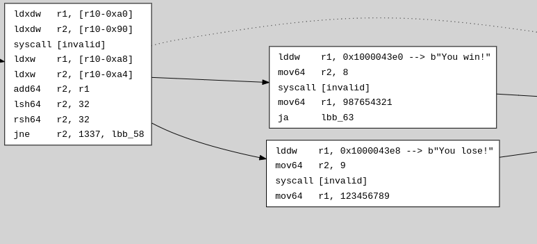
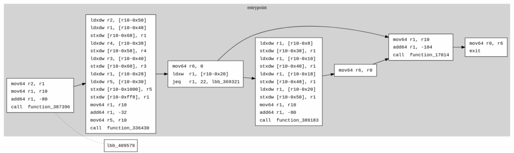
Beyond linear disassembly, sol-azy can reconstruct the program’s control flow graph, a directed graph that shows how execution flows through functions, basic blocks, and branches. The tool can output the CFG in Graphviz .dot format. This .dot file can be viewed as a diagram, illustrating nodes (basic blocks or functions) and edges (jumps or calls) that represent all possible execution paths. The CFG view is especially useful for complex programs with many branches, you can identify key decision points and see how different instructions lead to different outcomes. This feature works very well in combination with the dotting module (see “Other Features”) and the disassembly. It’s also worth noting that dynamic string resolution works for the CFG as well.
Still with the same code than above:
🌐
example_cfg.dot
... SNIP ...

lbb_58 [label=<<table border="0" cellpadding="3">
  <tr><td align="left">lddw</td><td align="left">r1, 0x1000043e8 --> b"You lose!"</td></tr>
  <tr><td align="left">mov64</td><td align="left">r2, 9</td></tr>
  <tr><td align="left">syscall</td><td align="left">[invalid]</td></tr>
  <tr><td align="left">mov64</td><td align="left">r1, 123456789</td></tr>
</table>>];

... SNIP ...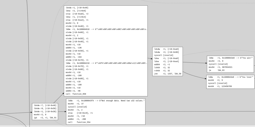
Also, the CFG module includes –reducedand–only-entrypoint options, which allow you to either reduce the CFG to just the main body of the program or limit it to its entrypoint only. (We’ll cover this later when presenting the Dotting module)
Rodata Extraction and Decoding
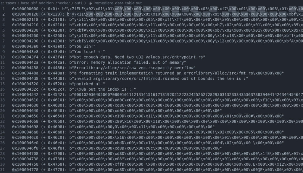
Solana programs often include embedded constants or strings in their read-only data segment (commonly called rodata). These might be error messages, program identifiers, or other magic values that are referenced by the code. sol-azy’s reverse engine automatically extracts and decodes the rodata from the binary and cross-references it in the disassembly output. In practice, this means when the assembly code loads a pointer to a string or constant, sol-azy will annotate the disassembly with the actual value (e.g., showing the literal error message or number). By tracking rodata usage, sol-azy gives more semantic context to the otherwise opaque assembly, you might immediately understand that a particular block of code is, say, the error handler for “Insufficient funds” just by seeing that string in the output.
Our immediate_data_table.out (with immediate referring to the offsets/addresses where the data resides in the bytecode):
Other Features: Build, Dotting, and Fetcher Modules
Aside from the core analysis engines, sol-azy includes additional features to support a full analysis workflow:
Build Module
build command is used to compile Solana programs from a specified project directory. It supports both Anchor and native SBF (Solana BPF) projects.
This feature is designed to automatically detect the project type (Anchor or SBF) based on the presence of specific files like Anchor.toml or solana-program in Cargo.toml, and it triggers the appropriate build command accordingly.
Key features:
- Simple usage via CLI (2 args, in/out directories)
- Pre-checks for required tools (cargo, anchor)
- Auto-creates output directories if needed
- Handles version switching with an optional flag
Note: The build feature is still in WIP
Dotting (CFG Editing) Module
The purpose of this module is to gradually reconstruct a meaningful CFG when analysing large programs, where the full graph can be overwhelming. When using the –reduced or –only-entrypoint flags during CFG generation, sol-azy outputs a minimal graph containing only a subset of functions (for example, only those reachable from the entrypoint or excluding library functions). The dotting module lets you then selectively re-insert specific functions (clusters) from the full graph into the reduced CFG. This workflow is useful during deep analysis: you start with a minimal graph and, as you explore the disassembly or identify relevant functions, you can progressively “grow” your graph by adding functions of interest. It’s particularly effective for large projects where the default full CFG is too dense to be practical. This feature is designed to be coupled with the –reduced or –only-entrypoint options to provide a flexible, iterative approach to CFG analysis.
—only-entrypointedit example (using the MangoV4 project, randomly chosen for the next part about a real-life example):
Before:
digraph {
graph [
rankdir=LR;
concentrate=True;
style=filled;
color=lightgrey;
];
node [
shape=rect;
style=filled;
fillcolor=white;
fontname="Courier New";
];
edge [
fontname="Courier New";
];
  subgraph cluster_369287 {
    label="entrypoint";
    tooltip=lbb_369287;
    lbb_369287 [label=<<table border="0" cellpadding="3"><tr><td align="left">mov64</td><td align="left">r2, r1</td></tr><tr><td align="left">mov64</td><td align="left">r1, r10</td></tr><tr><td align="left">add64</td><td align="left">r1, -80</td></tr><tr><td align="left">call</td><td align="left">function_387396</td></tr></table>>];
    lbb_369291 [label=<<table border="0" cellpadding="3"><tr><td align="left">ldxdw</td><td align="left">r2, [r10-0x50]</td></tr><tr><td align="left">ldxdw</td><td align="left">r1, [r10-0x48]</td></tr><tr><td align="left">stxdw</td><td align="left">[r10-0x68], r1</td></tr><tr><td align="left">ldxdw</td><td align="left">r4, [r10-0x38]</td></tr><tr><td align="left">stxdw</td><td align="left">[r10-0x58], r4</td></tr><tr><td align="left">ldxdw</td><td align="left">r3, [r10-0x40]</td></tr><tr><td align="left">stxdw</td><td align="left">[r10-0x60], r3</td></tr><tr><td align="left">ldxdw</td><td align="left">r1, [r10-0x28]</td></tr><tr><td align="left">ldxdw</td><td align="left">r5, [r10-0x30]</td></tr><tr><td align="left">stxdw</td><td align="left">[r10-0x1000], r5</td></tr><tr><td align="left">stxdw</td><td align="left">[r10-0xff8], r1</td></tr><tr><td align="left">mov64</td><td align="left">r1, r10</td></tr><tr><td align="left">add64</td><td align="left">r1, -32</td></tr><tr><td align="left">mov64</td><td align="left">r5, r10</td></tr><tr><td align="left">call</td><td align="left">function_336430</td></tr></table>>];
    lbb_369306 [label=<<table border="0" cellpadding="3"><tr><td align="left">mov64</td><td align="left">r6, 0</td></tr><tr><td align="left">ldxw</td><td align="left">r1, [r10-0x20]</td></tr><tr><td align="left">jeq</td><td align="left">r1, 22, lbb_369321</td></tr></table>>];
    lbb_369309 [label=<<table border="0" cellpadding="3"><tr><td align="left">ldxdw</td><td align="left">r1, [r10-0x8]</td></tr><tr><td align="left">stxdw</td><td align="left">[r10-0x38], r1</td></tr><tr><td align="left">ldxdw</td><td align="left">r1, [r10-0x10]</td></tr><tr><td align="left">stxdw</td><td align="left">[r10-0x40], r1</td></tr><tr><td align="left">ldxdw</td><td align="left">r1, [r10-0x18]</td></tr><tr><td align="left">stxdw</td><td align="left">[r10-0x48], r1</td></tr><tr><td align="left">ldxdw</td><td align="left">r1, [r10-0x20]</td></tr><tr><td align="left">stxdw</td><td align="left">[r10-0x50], r1</td></tr><tr><td align="left">mov64</td><td align="left">r1, r10</td></tr><tr><td align="left">add64</td><td align="left">r1, -80</td></tr><tr><td align="left">call</td><td align="left">function_389183</td></tr></table>>];
    lbb_369320 [label=<<table border="0" cellpadding="3"><tr><td align="left">mov64</td><td align="left">r6, r0</td></tr></table>>];
    lbb_369321 [label=<<table border="0" cellpadding="3"><tr><td align="left">mov64</td><td align="left">r1, r10</td></tr><tr><td align="left">add64</td><td align="left">r1, -104</td></tr><tr><td align="left">call</td><td align="left">function_17014</td></tr></table>>];
    lbb_369324 [label=<<table border="0" cellpadding="3"><tr><td align="left">mov64</td><td align="left">r0, r6</td></tr><tr><td align="left">exit</td></tr></table>>];
  }
  lbb_369287 -> lbb_409579 [style=dotted; arrowhead=none];
  lbb_369287 -> {lbb_369291};
  lbb_369291 -> lbb_369287 [style=dotted; arrowhead=none];
  lbb_369291 -> {lbb_369306};
  lbb_369306 -> lbb_369291 [style=dotted; arrowhead=none];
  lbb_369306 -> {lbb_369309 lbb_369321};
  lbb_369309 -> lbb_369306 [style=dotted; arrowhead=none];
  lbb_369309 -> {lbb_369320};
  lbb_369320 -> lbb_369309 [style=dotted; arrowhead=none];
  lbb_369320 -> {lbb_369321};
  lbb_369321 -> lbb_369306 [style=dotted; arrowhead=none];
  lbb_369321 -> {lbb_369324};
  lbb_369324 -> lbb_369321 [style=dotted; arrowhead=none];
}
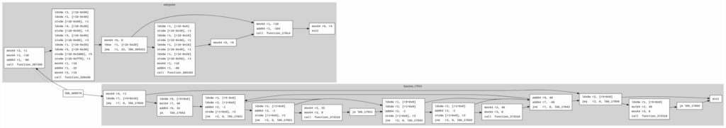
After adding a cluster:
digraph {
graph [
rankdir=LR;
concentrate=True;
style=filled;
color=lightgrey;
];
node [
shape=rect;
style=filled;
fillcolor=white;
fontname="Courier New";
];
edge [
fontname="Courier New";
];
  subgraph cluster_369287 {
    label="entrypoint";
    tooltip=lbb_369287;
    lbb_369287 [label=<<table border="0" cellpadding="3"><tr><td align="left">mov64</td><td align="left">r2, r1</td></tr><tr><td align="left">mov64</td><td align="left">r1, r10</td></tr><tr><td align="left">add64</td><td align="left">r1, -80</td></tr><tr><td align="left">call</td><td align="left">function_387396</td></tr></table>>];
    lbb_369291 [label=<<table border="0" cellpadding="3"><tr><td align="left">ldxdw</td><td align="left">r2, [r10-0x50]</td></tr><tr><td align="left">ldxdw</td><td align="left">r1, [r10-0x48]</td></tr><tr><td align="left">stxdw</td><td align="left">[r10-0x68], r1</td></tr><tr><td align="left">ldxdw</td><td align="left">r4, [r10-0x38]</td></tr><tr><td align="left">stxdw</td><td align="left">[r10-0x58], r4</td></tr><tr><td align="left">ldxdw</td><td align="left">r3, [r10-0x40]</td></tr><tr><td align="left">stxdw</td><td align="left">[r10-0x60], r3</td></tr><tr><td align="left">ldxdw</td><td align="left">r1, [r10-0x28]</td></tr><tr><td align="left">ldxdw</td><td align="left">r5, [r10-0x30]</td></tr><tr><td align="left">stxdw</td><td align="left">[r10-0x1000], r5</td></tr><tr><td align="left">stxdw</td><td align="left">[r10-0xff8], r1</td></tr><tr><td align="left">mov64</td><td align="left">r1, r10</td></tr><tr><td align="left">add64</td><td align="left">r1, -32</td></tr><tr><td align="left">mov64</td><td align="left">r5, r10</td></tr><tr><td align="left">call</td><td align="left">function_336430</td></tr></table>>];
    lbb_369306 [label=<<table border="0" cellpadding="3"><tr><td align="left">mov64</td><td align="left">r6, 0</td></tr><tr><td align="left">ldxw</td><td align="left">r1, [r10-0x20]</td></tr><tr><td align="left">jeq</td><td align="left">r1, 22, lbb_369321</td></tr></table>>];
    lbb_369309 [label=<<table border="0" cellpadding="3"><tr><td align="left">ldxdw</td><td align="left">r1, [r10-0x8]</td></tr><tr><td align="left">stxdw</td><td align="left">[r10-0x38], r1</td></tr><tr><td align="left">ldxdw</td><td align="left">r1, [r10-0x10]</td></tr><tr><td align="left">stxdw</td><td align="left">[r10-0x40], r1</td></tr><tr><td align="left">ldxdw</td><td align="left">r1, [r10-0x18]</td></tr><tr><td align="left">stxdw</td><td align="left">[r10-0x48], r1</td></tr><tr><td align="left">ldxdw</td><td align="left">r1, [r10-0x20]</td></tr><tr><td align="left">stxdw</td><td align="left">[r10-0x50], r1</td></tr><tr><td align="left">mov64</td><td align="left">r1, r10</td></tr><tr><td align="left">add64</td><td align="left">r1, -80</td></tr><tr><td align="left">call</td><td align="left">function_389183</td></tr></table>>];
    lbb_369320 [label=<<table border="0" cellpadding="3"><tr><td align="left">mov64</td><td align="left">r6, r0</td></tr></table>>];
    lbb_369321 [label=<<table border="0" cellpadding="3"><tr><td align="left">mov64</td><td align="left">r1, r10</td></tr><tr><td align="left">add64</td><td align="left">r1, -104</td></tr><tr><td align="left">call</td><td align="left">function_17014</td></tr></table>>];
    lbb_369324 [label=<<table border="0" cellpadding="3"><tr><td align="left">mov64</td><td align="left">r0, r6</td></tr><tr><td align="left">exit</td></tr></table>>];
  }
  lbb_369287 -> lbb_409579 [style=dotted; arrowhead=none];
  lbb_369287 -> {lbb_369291};
  lbb_369291 -> lbb_369287 [style=dotted; arrowhead=none];
  lbb_369291 -> {lbb_369306};
  lbb_369306 -> lbb_369291 [style=dotted; arrowhead=none];
  lbb_369306 -> {lbb_369309 lbb_369321};
  lbb_369309 -> lbb_369306 [style=dotted; arrowhead=none];
  lbb_369309 -> {lbb_369320};
  lbb_369320 -> lbb_369309 [style=dotted; arrowhead=none];
  lbb_369320 -> {lbb_369321};
  lbb_369321 -> lbb_369306 [style=dotted; arrowhead=none];
  lbb_369321 -> {lbb_369324};
  lbb_369324 -> lbb_369321 [style=dotted; arrowhead=none];

subgraph cluster_17014 {
    label="function_17014";
    tooltip=lbb_17014;
    lbb_17014 [label=<<table border="0" cellpadding="3"><tr><td align="left">mov64</td><td align="left">r6, r1</td></tr><tr><td align="left">ldxdw</td><td align="left">r7, [r6+0x10]</td></tr><tr><td align="left">jeq</td><td align="left">r7, 0, lbb_17036</td></tr></table>>];
    lbb_17017 [label=<<table border="0" cellpadding="3"><tr><td align="left">ldxdw</td><td align="left">r8, [r6+0x8]</td></tr><tr><td align="left">mul64</td><td align="left">r7, 48</td></tr><tr><td align="left">add64</td><td align="left">r8, 16</td></tr><tr><td align="left">ja</td><td align="left">lbb_17043</td></tr></table>>];
    lbb_17043 [label=<<table border="0" cellpadding="3"><tr><td align="left">ldxdw</td><td align="left">r1, [r8-0x8]</td></tr><tr><td align="left">ldxdw</td><td align="left">r2, [r1+0x0]</td></tr><tr><td align="left">add64</td><td align="left">r2, -1</td></tr><tr><td align="left">stxdw</td><td align="left">[r1+0x0], r2</td></tr><tr><td align="left">jne</td><td align="left">r2, 0, lbb_17021</td></tr></table>>];
    lbb_17048 [label=<<table border="0" cellpadding="3"><tr><td align="left">ldxdw</td><td align="left">r2, [r1+0x8]</td></tr><tr><td align="left">add64</td><td align="left">r2, -1</td></tr><tr><td align="left">stxdw</td><td align="left">[r1+0x8], r2</td></tr><tr><td align="left">jne</td><td align="left">r2, 0, lbb_17021</td></tr></table>>];
    lbb_17052 [label=<<table border="0" cellpadding="3"><tr><td align="left">mov64</td><td align="left">r2, 32</td></tr><tr><td align="left">mov64</td><td align="left">r3, 8</td></tr><tr><td align="left">call</td><td align="left">function_373318</td></tr></table>>];
    lbb_17055 [label=<<table border="0" cellpadding="3"><tr><td align="left">ja</td><td align="left">lbb_17021</td></tr></table>>];
    lbb_17021 [label=<<table border="0" cellpadding="3"><tr><td align="left">ldxdw</td><td align="left">r1, [r8+0x0]</td></tr><tr><td align="left">ldxdw</td><td align="left">r2, [r1+0x0]</td></tr><tr><td align="left">add64</td><td align="left">r2, -1</td></tr><tr><td align="left">stxdw</td><td align="left">[r1+0x0], r2</td></tr><tr><td align="left">jne</td><td align="left">r2, 0, lbb_17033</td></tr></table>>];
    lbb_17026 [label=<<table border="0" cellpadding="3"><tr><td align="left">ldxdw</td><td align="left">r2, [r1+0x8]</td></tr><tr><td align="left">add64</td><td align="left">r2, -1</td></tr><tr><td align="left">stxdw</td><td align="left">[r1+0x8], r2</td></tr><tr><td align="left">jne</td><td align="left">r2, 0, lbb_17033</td></tr></table>>];
    lbb_17030 [label=<<table border="0" cellpadding="3"><tr><td align="left">mov64</td><td align="left">r2, 40</td></tr><tr><td align="left">mov64</td><td align="left">r3, 8</td></tr><tr><td align="left">call</td><td align="left">function_373318</td></tr></table>>];
    lbb_17033 [label=<<table border="0" cellpadding="3"><tr><td align="left">add64</td><td align="left">r8, 48</td></tr><tr><td align="left">add64</td><td align="left">r7, -48</td></tr><tr><td align="left">jne</td><td align="left">r7, 0, lbb_17043</td></tr></table>>];
    lbb_17036 [label=<<table border="0" cellpadding="3"><tr><td align="left">ldxdw</td><td align="left">r2, [r6+0x0]</td></tr><tr><td align="left">jeq</td><td align="left">r2, 0, lbb_17056</td></tr></table>>];
    lbb_17038 [label=<<table border="0" cellpadding="3"><tr><td align="left">ldxdw</td><td align="left">r1, [r6+0x8]</td></tr><tr><td align="left">mul64</td><td align="left">r2, 48</td></tr><tr><td align="left">mov64</td><td align="left">r3, 8</td></tr><tr><td align="left">call</td><td align="left">function_373318</td></tr></table>>];
    lbb_17042 [label=<<table border="0" cellpadding="3"><tr><td align="left">ja</td><td align="left">lbb_17056</td></tr></table>>];
    lbb_17056 [label=<<table border="0" cellpadding="3"><tr><td align="left">exit</td></tr></table>>];
  }

lbb_17014 -> {lbb_17017 lbb_17036};
lbb_17017 -> {lbb_17043};
lbb_17021 -> {lbb_17026 lbb_17033};
lbb_17026 -> {lbb_17030 lbb_17033};
lbb_17030 -> {lbb_17033};
lbb_17033 -> {lbb_17036 lbb_17043};
lbb_17036 -> {lbb_17038 lbb_17056};
lbb_17038 -> {lbb_17042};
lbb_17042 -> {lbb_17056};
lbb_17043 -> {lbb_17021 lbb_17048};
lbb_17048 -> {lbb_17021 lbb_17052};
lbb_17052 -> {lbb_17055};
lbb_17055 -> {lbb_17021};
lbb_409579 -> {lbb_17014 lbb_369287};
}
Fetcher Module (On-Chain Bytecode & Data Retrieval)
By supplying a Solana program ID, the fetcher downloads the (on-chain) deployed bytecode and saves it locally as fetched_program.so. It also supports non-executable accounts, making it capable of dumping arbitrary on-chain data. Here’s how it works:
- Executable Accounts (Programs):
- The fetcher automatically detects whether the account is marked as executable.
- If the program uses the Upgradeable Loader (common on Solana), it transparently resolves the indirection to locate the actual
ProgramData. - It trims any unnecessary bytes before the ELF header and saves a clean
.sobinary ready for disassembly or reverse engineering.
- Non-Executable Accounts (AccountInfo):
- If the account isn’t executable, fetcher simply dumps the raw byte content to a
.binfile. - Fetch Anchor’s struct discriminator
- If the account isn’t executable, fetcher simply dumps the raw byte content to a
When dumping non-executable accounts, fetcher automatically prints the first 8 bytes of the data, which in Anchor programs typically corresponds to the discriminator (a hash uniquely identifying the struct type).
This provides hints about the account’s purpose and can be invaluable for auditing or reverse-engineering state accounts.
CLI Demo: Realistics Little Examples Command Flow
To illustrate how sol-azy can be used in practice, let’s walk through 2 scenarios that uses several of its features. First example, imagine you are a security auditor examining a Solana program, you only have the on-chain program ID. Secondly, let’s take the POV where the project has an open-source code on GitHub.
Black-box scenario
Firstly, you want to fetch the deployed bytecode. Here’s how you could do it with sol-azy:
cargo run --release -- fetcher -p 4MangoMjqJ2firMokCjjGgoK8d4MXcrgL7XJaL3w6fVg -o .This command dump from the blockchain the program’s ELF into a file named fetched_program.so. In one step, you’ve obtained the exact code running on-chain, without manually dealing with RPC calls.
Next, we use the reverse engineering engine to examine the binary. You can produce a reduced control flow graph, (here we only want the entrypoint cluster):
cargo run --release -- reverse \
  --mode cfg \
  --out-dir ./ \
  --bytecodes-file fetched_program.so  \
--labeling --only-entrypoint

mv cfg.dot cfg_reduced.dot # we'll use it later
Then we can both get disassembly and the full CFG (the full CFG will be used for dotting):
cargo run --release -- reverse \
  --mode both \
  --out-dir ./ \
  --bytecodes-file fetched_program.so  \
--labeling

# commands below just to simplify our life later
mv cfg.dot cfg_full.dot
dot -Tsvg cfg_reduced.dot > cfg_reduced.svg
Now let’s check about Immediate Tracking to inspect all constant data loaded via LD_* instructions, particularly .rodata strings embedded in the bytecode. As shown in the image below, it produces a clean table where every reference to such data is listed with its corresponding memory offset and decoded value. You can quickly scroll through this table to identify interesting strings, such as error messages, program paths, or even function identifiers, that might reveal sensitive logic or security-relevant checks.
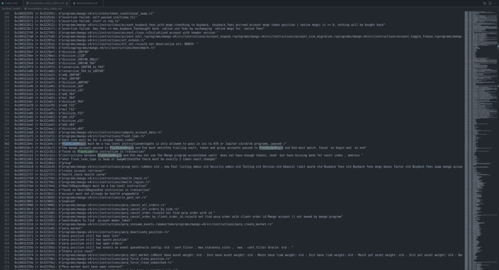
In the example above, you can clearly spot strings like “instructions between FlashLoanBegin and End may not use the Mango program accountbank vault” or “the mango account passed to FlashLoanBegin and End must matchthe trailing vault”. These strings provide immediate clues about the program’s behavior and potential areas of interest for further analysis. This makes the immediate tracking table a powerful reconnaissance tool, allowing you to locate critical logic areas without having to fully reverse the disassembly first.
Now we can just take a fast look at our disassembly, searching for things like the FlashLoan’s strings above, and we can find things like:
...

lbb_120970:
    mov64 r1, r9                                    r1 = r9
    lddw r2, 0x100326afa --> b"1\xd8\xe1}\xde\x0fY\xc1\x8e\x07[\x98\xca\x9dke\xc8\xfa$\xedPm l^\xbe b"\x00\x00\x00\x00\xc5\x09\x00\x00\x11\x00\x00\x00\x16\x00\x00\x00\xc8\x09\…        r2 load str located at 4298246740
    call function_334705
    mov64 r1, r10                                   r1 = r10
    add64 r1, -176                                  r1 += -176   ///  r1 = r1.wrapping_add(-176 as i32 as i64 as u64)
    lddw r2, 0x100320a54 --> b"\x00\x00\x00\x00\xc5\x09\x00\x00\x11\x00\x00\x00\x16\x00\x00\x00\xc8\x09\…        r2 load str located at 4298246740
    call function_10004
    mov64 r1, 2                                     r1 = 2 as i32 as i64 as u64
    stxb [r10-0x98], r1
    mov64 r1, 185                                   r1 = 185 as i32 as i64 as u64
    stxw [r10-0xd0], r1
    mov64 r1, 48                                    r1 = 48 as i32 as i64 as u64
    stxdw [r10-0xd8], r1
    lddw r1, 0x100322af2 --> b"programs/mango-v4/src/instructions/flash_loan.rsea"        r1 load str located at 4298255090
    stxdw [r10-0xe0], r1
    mov64 r1, 6000                                  r1 = 6000 as i32 as i64 as u64
    stxw [r10-0x50], r1
    mov64 r6, 0                                     r6 = 0 as i32 as i64 as u64
    stxdw [r10-0xe8], r6
    mov64 r7, r10                                   r7 = r10
    add64 r7, -800                                  r7 += -800   ///  r7 = r7.wrapping_add(-800 as i32 as i64 as u64)
    mov64 r2, r10                                   r2 = r10
    add64 r2, -232                                  r2 += -232   ///  r2 = r2.wrapping_add(-232 as i32 as i64 as u64)
    mov64 r1, r7                                    r1 = r7
    call function_384657
    mov64 r1, 1                                     r1 = 1 as i32 as i64 as u64
    stxdw [r10-0xd0], r1
    lddw r1, 0x10032fbc8 --> b"\x00\x00\x00\x00\xb1,2\x00Q\x00\x00\x00\x00\x00\x00\x00\x00\x00\x00\x00\x…        r1 load str located at 4298308552
    stxdw [r10-0xd8], r1
    lddw r1, 0x100320150 --> b"\x04y\xd5-\xed\xbfk\xc5\xec\xd0\x9d\x84SJ4\xae\xa5\x97PC\xb3o\xd0+$e\x0b\…        r1 load str located at 4298244432
    stxdw [r10-0xc8], r1
    stxdw [r10-0xc0], r6
    stxdw [r10-0xe8], r6
    mov64 r6, r10                                   r6 = r10
    add64 r6, -384                                  r6 += -384   ///  r6 = r6.wrapping_add(-384 as i32 as i64 as u64)
    mov64 r4, r10                                   r4 = r10
    add64 r4, -232                                  r4 += -232   ///  r4 = r4.wrapping_add(-232 as i32 as i64 as u64)
    mov64 r1, r6                                    r1 = r6
    lddw r2, 0x100322cb1 --> b"instructions between FlashLoanBegin and End may not use the Mango program…        r2 load str located at 4298255537
    mov64 r3, 81                                    r3 = 81 as i32 as i64 as u64
    ja lbb_121774

    ...
In this example, the disassembly clearly shows that the instruction sequence is tied to flash loan security checks. (might be an interesting point for research)
Now: Interactive CFG Editing (advanced). We’re with our reduced control flow graph that was generated using the –only-entrypoint flag. This gives us a minimal view of the program’s structure, usually limited to just the entrypoint function.
dot -Tsvg cfg_reduced.dot > cfg_reduced.svg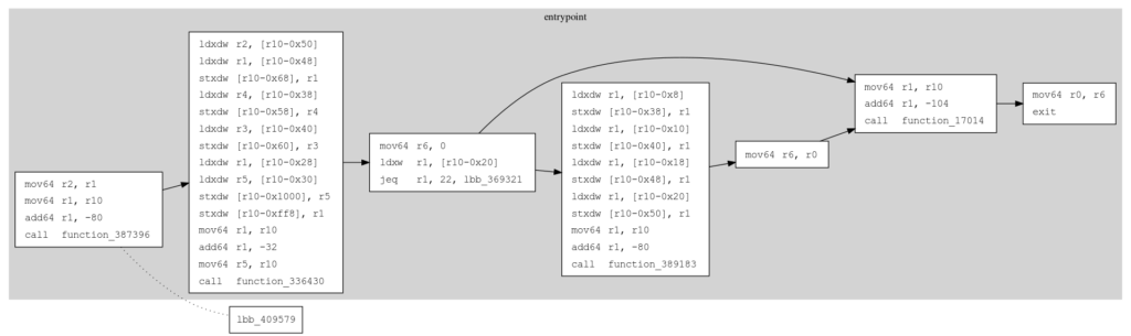
At this stage, when opening cfg_reduced.svg, we observe that only a single cluster, corresponding to the entrypoint, is present.
Upon inspection of the disassembly or node labels, we see that this entrypoint function invokes
function_17014at the end.
Since function_17014 is not currently included in the reduced graph, we decide to manually add it back using the dotting module. We create a small JSON configuration file specifying the ID of the cluster we want to re-insert:
// functions.json
{
    "functions": ["17014"]
}
Now we run the dotting command, which compares the reduced and full .dot files, and 17014, including any edges that are compatible with the existing graph:
cargo run --release -- dotting -c functions.json -f cfg_full.dot -r cfg_reduced.dotAfter this operation, the tool produces a new file named updated_cfg_reduced.dot. It contains the original reduced CFG plus the full definition of function_17014 as extracted from the complete graph.
Finally, we render the updated graph to see the result:
dot -Tsvg updated_cfg_reduced.dot > cfg_updated.svgOpening cfg_updated.svg, we can now see that function_17014 has been successfully added. This expanded view allows us to analyze the callee’s logic in context, without needing to visualize the entire program.
We can repeat this process iteratively to construct a CFG tailored to the parts of the program that are relevant to our analysis.
This workflow illustrates how dotting acts as a controlled lens, giving you the power to build up your graph gradually as your investigation progresses.
Note: The dotting module includes an internal cache system. After the first execution, subsequent runs become almost instantaneous, even on large .dot files, dramatically improving iteration speed during interactive analysis.
White-Box scenario
Now, we can clone the source code of mango and run the sast option on it.
git clone https://github.com/blockworks-foundation/mango-v4
cd sol-azy
cargo run --release -- sast --target-dir ../mango-v4/programs/mango-v4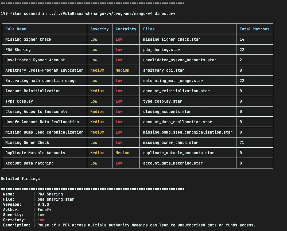
Then you can triage the matches found during the scan, for example in the Saturating math operation usage results:
Matches found: 22
...
../../VulnResearch/mango-v4/programs/mango-v4/src/health/client.rs:79:31
...
We got this sink
🦀
client.rs
...
    fn apply_limits_to_swap(
        account: &MangoAccountValue,
        source_bank: &Bank,
        source_oracle_price: I80F48,
        target_bank: &Bank,
        price: I80F48,
        source_unlimited: I80F48,
    ) -> Result {
        ...
        // deposit limit on target
        let available_deposits = target_bank.remaining_deposits_until_limit();
        let potential_target_unlimited = potential_source.saturating_mul(price);
        let potential_target = potential_target_unlimited
            .min(available_deposits.saturating_add(-target_pos.min(I80F48::ZERO)));
	...
    }
...
Conclusion: Why sol-azy Matters, Who Should Use It, and What’s Next
In conclusion, sol-azy offers a powerful and unified solution for anyone working with Solana programs, from security auditors to new developers. By bringing together static analysis, reverse engineering capabilities, and convenient on-chain data retrieval into a single CLI toolkit.
Whether you’re verifying the security of closed-source programs, dissecting complex bytecode, or auditing deployed contracts, sol-azy provides the essential tools to understand and interact with Solana’s unique program ecosystem on your terms.
sol-azy is an early version, but we’ve got big plans to make it even better:
- Finish Build Command: We’re working to make the
buildcommand smoother and more flexible for all Solana project types. - Smarter Static Analysis: Our static analysis engine is getting an upgrade. We’ll add more ways to write rules and support analyzing other intermediate representations like MIR and LLVM IR for even deeper insights.
- And more
Your feedback and contributions are always welcome as we keep building it out.
References
Dimitri C. / @Ectari0
Mohammed B.
About Us
Founded in 2021 and headquartered in Paris, FuzzingLabs is a cybersecurity startup specializing in vulnerability research, fuzzing, and blockchain security. We combine cutting-edge research with hands-on expertise to secure some of the most critical components in the blockchain ecosystem.
Contact us for an audit or long term partnership!